0. 環(huán)境介紹
Python 版 本： 3.6.2
操作系統(tǒng)　　： Windows
集成開發(fā)環(huán)境： PyCharm
1. 安裝Python環(huán)境
安裝Python
首先，我們需要安裝Python環(huán)境。本人選擇的是64位版本的Python 3.6.2。去Python官網(wǎng)https://www.python.org/選擇相應(yīng)的版本并下載。如下如所示：

接下來安裝，并最終選擇將Python加入環(huán)境變量中。
安裝依賴包
去網(wǎng)址：http://www.lfd.uci.edu/~gohlke/pythonlibs/中去下載你所需要的如下Python安裝包：
?numpy-1.13.1+mkl-cp36-cp36m-win_amd64.whl
?scipy-0.19.1-cp36-cp36m-win_amd64.whl
?xgboost-0.6-cp36-cp36m-win_amd64.whl
1
2
3
假設(shè)上述三個(gè)包所在的目錄為D:\Application，則運(yùn)行Windows 命令行運(yùn)行程序cmd，并將當(dāng)前目錄轉(zhuǎn)到這兩個(gè)文件所在的目錄下。并依次執(zhí)行如下操作安裝這兩個(gè)包：

>> pip install numpy-1.13.1+mkl-cp36-cp36m-win_amd64.whl
>> pip install scipy-0.19.1-cp36-cp36m-win_amd64.whl
>> pip install xgboost-0.6-cp36-cp36m-win_amd64.whl
1
2
3
安裝Scikit-learn

眾所周知，scikit-learn是Python機(jī)器學(xué)習(xí)最著名的開源庫之一。因此，我們需要安裝此庫。執(zhí)行如下命令安裝scikit-learn機(jī)器學(xué)習(xí)庫：

>> pip install -U scikit-learn
1
測試安裝是否成功
>>> from sklearn import svm
>>> X = [[0, 0], [1, 1]]
>>> y = [0, 1]
>>> clf = svm.SVC()
>>> clf.fit(X, y) ?
>>> clf.predict([[2., 2.]])
array([1])
>>> import xgboost as xgb
1
2
3
4
5
6
7
8
注意：如果如上所述正確輸出，則表示安裝完成。否則就需要檢查安裝步驟是否出錯(cuò)，或者系統(tǒng)是否缺少必要的Windows依賴庫。常用的一般情況會(huì)出現(xiàn)缺少VC++運(yùn)行庫，在Windows 7、8、10等版本中安裝Visual C++ 2015基本上就能解決問題。

安裝PyCharm

對(duì)于PyChram的下載，請(qǐng)點(diǎn)擊PyCharm官網(wǎng)去下載，當(dāng)然windows下軟件的安裝不用解釋，傻瓜式的點(diǎn)擊 下一步 就行了。

注意：PyCharm軟件是基于Java開發(fā)的，所以安裝該集成開發(fā)環(huán)境前請(qǐng)先安裝JDK，建議安裝JDK1.8。

經(jīng)過上述步驟，基本上軟件環(huán)境的問題全部解決了，接下來就是實(shí)際的XGBoost庫實(shí)戰(zhàn)了……

2. XGBoost的優(yōu)點(diǎn)
2.1 正則化
XGBoost在代價(jià)函數(shù)里加入了正則項(xiàng)，用于控制模型的復(fù)雜度。正則項(xiàng)里包含了樹的葉子節(jié)點(diǎn)個(gè)數(shù)、每個(gè)葉子節(jié)點(diǎn)上輸出的score的L2模的平方和。從Bias-variance tradeoff角度來講，正則項(xiàng)降低了模型的variance，使學(xué)習(xí)出來的模型更加簡單，防止過擬合，這也是xgboost優(yōu)于傳統(tǒng)GBDT的一個(gè)特性。

2.2 并行處理
XGBoost工具支持并行。Boosting不是一種串行的結(jié)構(gòu)嗎?怎么并行的？注意XGBoost的并行不是tree粒度的并行，XGBoost也是一次迭代完才能進(jìn)行下一次迭代的（第t次迭代的代價(jià)函數(shù)里包含了前面t-1次迭代的預(yù)測值）。XGBoost的并行是在特征粒度上的。

我們知道，決策樹的學(xué)習(xí)最耗時(shí)的一個(gè)步驟就是對(duì)特征的值進(jìn)行排序（因?yàn)橐_定最佳分割點(diǎn)），XGBoost在訓(xùn)練之前，預(yù)先對(duì)數(shù)據(jù)進(jìn)行了排序，然后保存為block結(jié)構(gòu)，后面的迭代中重復(fù)地使用這個(gè)結(jié)構(gòu)，大大減小計(jì)算量。這個(gè)block結(jié)構(gòu)也使得并行成為了可能，在進(jìn)行節(jié)點(diǎn)的分裂時(shí)，需要計(jì)算每個(gè)特征的增益，最終選增益最大的那個(gè)特征去做分裂，那么各個(gè)特征的增益計(jì)算就可以開多線程進(jìn)行。

2.3 靈活性
XGBoost支持用戶自定義目標(biāo)函數(shù)和評(píng)估函數(shù)，只要目標(biāo)函數(shù)二階可導(dǎo)就行。

2.4 缺失值處理
對(duì)于特征的值有缺失的樣本，xgboost可以自動(dòng)學(xué)習(xí)出它的分裂方向

2.5 剪枝
XGBoost 先從頂?shù)降捉⑺锌梢越⒌淖訕?#xff0c;再從底到頂反向進(jìn)行剪枝。比起GBM，這樣不容易陷入局部最優(yōu)解。

2.6 內(nèi)置交叉驗(yàn)證
XGBoost允許在每一輪boosting迭代中使用交叉驗(yàn)證。因此，可以方便地獲得最優(yōu)boosting迭代次數(shù)。而GBM使用網(wǎng)格搜索，只能檢測有限個(gè)值。

3. XGBoost詳解
3.1 數(shù)據(jù)格式
XGBoost可以加載多種數(shù)據(jù)格式的訓(xùn)練數(shù)據(jù)：

libsvm 格式的文本數(shù)據(jù)；

Numpy 的二維數(shù)組；

XGBoost 的二進(jìn)制的緩存文件。加載的數(shù)據(jù)存儲(chǔ)在對(duì)象 **DMatrix **中。

下面一一列舉：

加載libsvm格式的數(shù)據(jù)
>>> dtrain1 = xgb.DMatrix('train.svm.txt')
1
加載二進(jìn)制的緩存文件
>>> dtrain2 = xgb.DMatrix('train.svm.buffer')
1
加載numpy的數(shù)組
>>> data = np.random.rand(5,10) # 5 entities, each contains 10 features
>>> label = np.random.randint(2, size=5) # binary target
>>> dtrain = xgb.DMatrix( data, label=label)
1
2
3
將scipy.sparse格式的數(shù)據(jù)轉(zhuǎn)化為 DMatrix 格式
>>> csr = scipy.sparse.csr_matrix( (dat, (row,col)) )
>>> dtrain = xgb.DMatrix( csr )
1
2
將 DMatrix 格式的數(shù)據(jù)保存成XGBoost的二進(jìn)制格式，在下次加載時(shí)可以提高加載速度，使用方式如下
>>> dtrain = xgb.DMatrix('train.svm.txt')
>>> dtrain.save_binary("train.buffer")
1
2
可以用如下方式處理 DMatrix中的缺失值：
>>> dtrain = xgb.DMatrix( data, label=label, missing = -999.0)
1
當(dāng)需要給樣本設(shè)置權(quán)重時(shí)，可以用如下方式
>>> w = np.random.rand(5,1)
>>> dtrain = xgb.DMatrix( data, label=label, missing = -999.0, weight=w)
1
2
3.2 參數(shù)設(shè)置
XGBoost使用key-value字典的方式存儲(chǔ)參數(shù)：

params = {
? ? 'booster': 'gbtree',
? ? 'objective': 'multi:softmax', ?# 多分類的問題
? ? 'num_class': 10, ? ? ? ? ? ? ? # 類別數(shù)，與 multisoftmax 并用
? ? 'gamma': 0.1, ? ? ? ? ? ? ? ? ?# 用于控制是否后剪枝的參數(shù),越大越保守，一般0.1、0.2這樣子。
? ? 'max_depth': 12, ? ? ? ? ? ? ? # 構(gòu)建樹的深度，越大越容易過擬合
? ? 'lambda': 2, ? ? ? ? ? ? ? ? ? # 控制模型復(fù)雜度的權(quán)重值的L2正則化項(xiàng)參數(shù)，參數(shù)越大，模型越不容易過擬合。
? ? 'subsample': 0.7, ? ? ? ? ? ? ?# 隨機(jī)采樣訓(xùn)練樣本
? ? 'colsample_bytree': 0.7, ? ? ? # 生成樹時(shí)進(jìn)行的列采樣
? ? 'min_child_weight': 3,
? ? 'silent': 1, ? ? ? ? ? ? ? ? ? # 設(shè)置成1則沒有運(yùn)行信息輸出，最好是設(shè)置為0.
? ? 'eta': 0.007, ? ? ? ? ? ? ? ? ?# 如同學(xué)習(xí)率
? ? 'seed': 1000,
? ? 'nthread': 4, ? ? ? ? ? ? ? ? ?# cpu 線程數(shù)
}
1
2
3
4
5
6
7
8
9
10
11
12
13
14
15
3.3 訓(xùn)練模型
有了參數(shù)列表和數(shù)據(jù)就可以訓(xùn)練模型了

num_round = 10
bst = xgb.train( plst, dtrain, num_round, evallist )
1
2
3.4 模型預(yù)測
# X_test類型可以是二維List，也可以是numpy的數(shù)組
dtest = DMatrix(X_test)
ans = model.predict(dtest)
1
2
3
3.5 保存模型
在訓(xùn)練完成之后可以將模型保存下來，也可以查看模型內(nèi)部的結(jié)構(gòu)
? ? bst.save_model('test.model')
1
導(dǎo)出模型和特征映射（Map）
你可以導(dǎo)出模型到txt文件并瀏覽模型的含義：

# dump model
bst.dump_model('dump.raw.txt')
# dump model with feature map
bst.dump_model('dump.raw.txt','featmap.txt')
1
2
3
4
3.6 加載模型
通過如下方式可以加載模型：

bst = xgb.Booster({'nthread':4}) # init model
bst.load_model("model.bin") ? ? ?# load data
1
2
4. XGBoost參數(shù)詳解
在運(yùn)行XGboost之前，必須設(shè)置三種類型成熟：general parameters，booster parameters和task parameters：

General parameters
該參數(shù)參數(shù)控制在提升（boosting）過程中使用哪種booster，常用的booster有樹模型（tree）和線性模型（linear model）。

Booster parameters
這取決于使用哪種booster。

Task parameters
控制學(xué)習(xí)的場景，例如在回歸問題中會(huì)使用不同的參數(shù)控制排序。

4.1 General Parameters
booster [default=gbtree]
有兩中模型可以選擇gbtree和gblinear。gbtree使用基于樹的模型進(jìn)行提升計(jì)算，gblinear使用線性模型進(jìn)行提升計(jì)算。缺省值為gbtree

silent [default=0]
取0時(shí)表示打印出運(yùn)行時(shí)信息，取1時(shí)表示以緘默方式運(yùn)行，不打印運(yùn)行時(shí)信息。缺省值為0

**nthread **
XGBoost運(yùn)行時(shí)的線程數(shù)。缺省值是當(dāng)前系統(tǒng)可以獲得的最大線程數(shù)

num_pbuffer
預(yù)測緩沖區(qū)大小，通常設(shè)置為訓(xùn)練實(shí)例的數(shù)目。緩沖用于保存最后一步提升的預(yù)測結(jié)果，無需人為設(shè)置。

**num_feature **
Boosting過程中用到的特征維數(shù)，設(shè)置為特征個(gè)數(shù)。XGBoost會(huì)自動(dòng)設(shè)置，無需人為設(shè)置。

4.2 Parameters for Tree Booster
eta [default=0.3]
為了防止過擬合，更新過程中用到的收縮步長。在每次提升計(jì)算之后，算法會(huì)直接獲得新特征的權(quán)重。 eta通過縮減特征的權(quán)重使提升計(jì)算過程更加保守。缺省值為0.3
取值范圍為：[0,1]

gamma [default=0]
minimum loss reduction required to make a further partition on a leaf node of the tree. the larger, the more conservative the algorithm will be.
取值范圍為：[0,∞]

max_depth [default=6]
數(shù)的最大深度。缺省值為6
取值范圍為：[1,∞]

min_child_weight [default=1]
孩子節(jié)點(diǎn)中最小的樣本權(quán)重和。如果一個(gè)葉子節(jié)點(diǎn)的樣本權(quán)重和小于min_child_weight則拆分過程結(jié)束。在現(xiàn)行回歸模型中，這個(gè)參數(shù)是指建立每個(gè)模型所需要的最小樣本數(shù)。該成熟越大算法越conservative
取值范圍為：[0,∞]

max_delta_step [default=0]
我們?cè)试S每個(gè)樹的權(quán)重被估計(jì)的值。如果它的值被設(shè)置為0，意味著沒有約束；如果它被設(shè)置為一個(gè)正值，它能夠使得更新的步驟更加保守。通常這個(gè)參數(shù)是沒有必要的，但是如果在邏輯回歸中類極其不平衡這時(shí)候他有可能會(huì)起到幫助作用。把它范圍設(shè)置為1-10之間也許能控制更新。
取值范圍為：[0,∞]

subsample [default=1]
用于訓(xùn)練模型的子樣本占整個(gè)樣本集合的比例。如果設(shè)置為0.5則意味著XGBoost將隨機(jī)的從整個(gè)樣本集合中隨機(jī)的抽取出50%的子樣本建立樹模型，這能夠防止過擬合。
取值范圍為：(0,1]

colsample_bytree [default=1]
在建立樹時(shí)對(duì)特征采樣的比例。缺省值為1
取值范圍為：(0,1]

4.3 Parameter for Linear Booster
lambda [default=0]
L2 正則的懲罰系數(shù)

alpha [default=0]
L1 正則的懲罰系數(shù)

lambda_bias
在偏置上的L2正則。缺省值為0（在L1上沒有偏置項(xiàng)的正則，因?yàn)長1時(shí)偏置不重要）

4.4 Task Parameters
objective [ default=reg:linear ]
定義學(xué)習(xí)任務(wù)及相應(yīng)的學(xué)習(xí)目標(biāo)，可選的目標(biāo)函數(shù)如下：

“reg:linear” —— 線性回歸。

“reg:logistic”—— 邏輯回歸。

“binary:logistic”—— 二分類的邏輯回歸問題，輸出為概率。

“binary:logitraw”—— 二分類的邏輯回歸問題，輸出的結(jié)果為wTx。

“count:poisson”—— 計(jì)數(shù)問題的poisson回歸，輸出結(jié)果為poisson分布。在poisson回歸中，max_delta_step的缺省值為0.7。(used to safeguard optimization)

“multi:softmax” –讓XGBoost采用softmax目標(biāo)函數(shù)處理多分類問題，同時(shí)需要設(shè)置參數(shù)num_class（類別個(gè)數(shù)）

“multi:softprob” –和softmax一樣，但是輸出的是ndata * nclass的向量，可以將該向量reshape成ndata行nclass列的矩陣。沒行數(shù)據(jù)表示樣本所屬于每個(gè)類別的概率。

“rank:pairwise” –set XGBoost to do ranking task by minimizing the pairwise loss

base_score [ default=0.5 ]

所有實(shí)例的初始化預(yù)測分?jǐn)?shù)，全局偏置；
為了足夠的迭代次數(shù)，改變這個(gè)值將不會(huì)有太大的影響。
eval_metric [ default according to objective ]

校驗(yàn)數(shù)據(jù)所需要的評(píng)價(jià)指標(biāo)，不同的目標(biāo)函數(shù)將會(huì)有缺省的評(píng)價(jià)指標(biāo)（rmse for regression, and error for classification, mean average precision for ranking）-

用戶可以添加多種評(píng)價(jià)指標(biāo)，對(duì)于Python用戶要以list傳遞參數(shù)對(duì)給程序，而不是map參數(shù)list參數(shù)不會(huì)覆蓋’eval_metric’

可供的選擇如下:

“rmse”: root mean square error
“l(fā)ogloss”: negative log-likelihood
“error”: Binary classification error rate. It is calculated as #(wrong cases)/#(all cases). For the predictions, the evaluation will regard the instances with prediction value larger than 0.5 as positive instances, and the others as negative instances.
“merror”: Multiclass classification error rate. It is calculated as #(wrongcases)#(allcases)\frac{\#(wrong \quad cases)}{\#(all \quad cases)}?
#(allcases)
#(wrongcases)
??? ?
?.
“mlogloss”: Multiclass logloss
“auc”: Area under the curve for ranking evaluation.
“ndcg”:Normalized Discounted Cumulative Gain
“map”:Mean average precision
“ndcg@n”,”map@n”: n can be assigned as an integer to cut off the top positions in the lists for evaluation.
“ndcg-“,”map-“,”ndcg@n-“,”map@n-“: In XGBoost, NDCG and MAP will evaluate the score of a list without any positive samples as 1. By adding “-” in the evaluation metric XGBoost will evaluate these score as 0 to be consistent under some conditions. training repeatively
seed [ default=0 ]

隨機(jī)數(shù)的種子。缺省值為0
5. XGBoost實(shí)戰(zhàn)
XGBoost有兩大類接口：XGBoost原生接口 和 scikit-learn接口 ，并且XGBoost能夠?qū)崿F(xiàn) 分類 和 回歸 兩種任務(wù)。因此，本章節(jié)分四個(gè)小塊來介紹！

5.1 基于XGBoost原生接口的分類
from sklearn.datasets import load_iris
import xgboost as xgb
from xgboost import plot_importance
from matplotlib import pyplot as plt
from sklearn.model_selection import train_test_split

# read in the iris data
iris = load_iris()

X = iris.data
y = iris.target

X_train, X_test, y_train, y_test = train_test_split(X, y, test_size=0.2, random_state=1234565)

params = {
? ? 'booster': 'gbtree',
? ? 'objective': 'multi:softmax',
? ? 'num_class': 3,
? ? 'gamma': 0.1,
? ? 'max_depth': 6,
? ? 'lambda': 2,
? ? 'subsample': 0.7,
? ? 'colsample_bytree': 0.7,
? ? 'min_child_weight': 3,
? ? 'silent': 1,
? ? 'eta': 0.1,
? ? 'seed': 1000,
? ? 'nthread': 4,
}

plst = params.items()

dtrain = xgb.DMatrix(X_train, y_train)
num_rounds = 500
model = xgb.train(plst, dtrain, num_rounds)

# 對(duì)測試集進(jìn)行預(yù)測
dtest = xgb.DMatrix(X_test)
ans = model.predict(dtest)

# 計(jì)算準(zhǔn)確率
cnt1 = 0
cnt2 = 0
for i in range(len(y_test)):
? ? if ans[i] == y_test[i]:
? ? ? ? cnt1 += 1
? ? else:
? ? ? ? cnt2 += 1

print("Accuracy: %.2f %% " % (100 * cnt1 / (cnt1 + cnt2)))

# 顯示重要特征
plot_importance(model)
plt.show()

1
2
3
4
5
6
7
8
9
10
11
12
13
14
15
16
17
18
19
20
21
22
23
24
25
26
27
28
29
30
31
32
33
34
35
36
37
38
39
40
41
42
43
44
45
46
47
48
49
50
51
52
53
54
55
56
輸出預(yù)測正確率以及特征重要性：

Accuracy: 96.67 %?
1
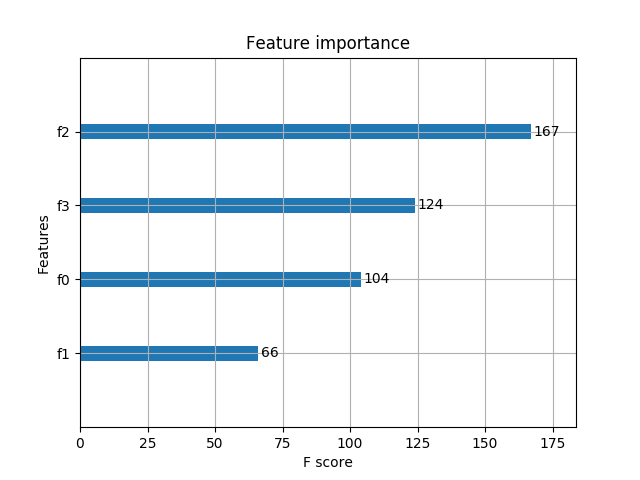
5.2 基于XGBoost原生接口的回歸
import xgboost as xgb
from xgboost import plot_importance
from matplotlib import pyplot as plt
from sklearn.model_selection import train_test_split

# 讀取文件原始數(shù)據(jù)
data = []
labels = []
labels2 = []
with open("lppz5.csv", encoding='UTF-8') as fileObject:
? ? for line in fileObject:
? ? ? ? line_split = line.split(',')
? ? ? ? data.append(line_split[10:])
? ? ? ? labels.append(line_split[8])

X = []
for row in data:
? ? row = [float(x) for x in row]
? ? X.append(row)

y = [float(x) for x in labels]

# XGBoost訓(xùn)練過程
X_train, X_test, y_train, y_test = train_test_split(X, y, test_size=0.2, random_state=0)

params = {
? ? 'booster': 'gbtree',
? ? 'objective': 'reg:gamma',
? ? 'gamma': 0.1,
? ? 'max_depth': 5,
? ? 'lambda': 3,
? ? 'subsample': 0.7,
? ? 'colsample_bytree': 0.7,
? ? 'min_child_weight': 3,
? ? 'silent': 1,
? ? 'eta': 0.1,
? ? 'seed': 1000,
? ? 'nthread': 4,
}

dtrain = xgb.DMatrix(X_train, y_train)
num_rounds = 300
plst = params.items()
model = xgb.train(plst, dtrain, num_rounds)

# 對(duì)測試集進(jìn)行預(yù)測
dtest = xgb.DMatrix(X_test)
ans = model.predict(dtest)

# 顯示重要特征
plot_importance(model)
plt.show()
1
2
3
4
5
6
7
8
9
10
11
12
13
14
15
16
17
18
19
20
21
22
23
24
25
26
27
28
29
30
31
32
33
34
35
36
37
38
39
40
41
42
43
44
45
46
47
48
49
50
51
52
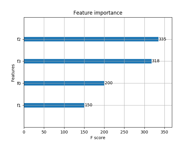
重要特征(值越大，說明該特征越重要)顯示結(jié)果：

5.3 基于Scikit-learn接口的分類
from sklearn.datasets import load_iris
import xgboost as xgb
from xgboost import plot_importance
from matplotlib import pyplot as plt
from sklearn.model_selection import train_test_split

# read in the iris data
iris = load_iris()

X = iris.data
y = iris.target

X_train, X_test, y_train, y_test = train_test_split(X, y, test_size=0.2, random_state=0)

# 訓(xùn)練模型
model = xgb.XGBClassifier(max_depth=5, learning_rate=0.1, n_estimators=160, silent=True, objective='multi:softmax')
model.fit(X_train, y_train)

# 對(duì)測試集進(jìn)行預(yù)測
ans = model.predict(X_test)

# 計(jì)算準(zhǔn)確率
cnt1 = 0
cnt2 = 0
for i in range(len(y_test)):
? ? if ans[i] == y_test[i]:
? ? ? ? cnt1 += 1
? ? else:
? ? ? ? cnt2 += 1

print("Accuracy: %.2f %% " % (100 * cnt1 / (cnt1 + cnt2)))

# 顯示重要特征
plot_importance(model)
plt.show()
1
2
3
4
5
6
7
8
9
10
11
12
13
14
15
16
17
18
19
20
21
22
23
24
25
26
27
28
29
30
31
32
33
34
35
輸出預(yù)測正確率以及特征重要性：

Accuracy: 100.00 %?
1
5.4 基于Scikit-learn接口的回歸
import xgboost as xgb
from xgboost import plot_importance
from matplotlib import pyplot as plt
from sklearn.model_selection import train_test_split

# 讀取文件原始數(shù)據(jù)
data = []
labels = []
labels2 = []
with open("lppz5.csv", encoding='UTF-8') as fileObject:
? ? for line in fileObject:
? ? ? ? line_split = line.split(',')
? ? ? ? data.append(line_split[10:])
? ? ? ? labels.append(line_split[8])

X = []
for row in data:
? ? row = [float(x) for x in row]
? ? X.append(row)

y = [float(x) for x in labels]

# XGBoost訓(xùn)練過程
X_train, X_test, y_train, y_test = train_test_split(X, y, test_size=0.2, random_state=0)

model = xgb.XGBRegressor(max_depth=5, learning_rate=0.1, n_estimators=160, silent=True, objective='reg:gamma')
model.fit(X_train, y_train)

# 對(duì)測試集進(jìn)行預(yù)測
ans = model.predict(X_test)

# 顯示重要特征
plot_importance(model)
plt.show()
1
2
3
4
5
6
7
8
9
10
11
12
13
14
15
16
17
18
19
20
21
22
23
24
25
26
27
28
29
30
31
32
33
34
重要特征(值越大，說明該特征越重要)顯示結(jié)果：

未完待續(xù)……

對(duì)機(jī)器學(xué)習(xí)和人工智能感興趣，請(qǐng)微信掃碼關(guān)注公眾號(hào)！
————————————————
版權(quán)聲明：本文為CSDN博主「JeemyJohn」的原創(chuàng)文章，遵循 CC 4.0 BY-SA 版權(quán)協(xié)議，轉(zhuǎn)載請(qǐng)附上原文出處鏈接及本聲明。
原文鏈接：https://blog.csdn.net/u013709270/article/details/78156207

與50位技術(shù)專家面對(duì)面20年技術(shù)見證，附贈(zèng)技術(shù)全景圖

總結(jié)

以上是生活随笔為你收集整理的史上最详细的XGBoost实战的全部內(nèi)容，希望文章能夠幫你解決所遇到的問題。

如果覺得生活随笔網(wǎng)站內(nèi)容還不錯(cuò)，歡迎將生活随笔推薦給好友。